A simple case of Dimensionality Reduction
A list of 10 points is an example of a two-dimensional dataset. We can plot this data set to look for a trend
| X - Value | Y - Value |
|---|---|
| 0.03 | 0.10 |
| 0.56 | 0.50 |
| 0.88 | 0.73 |
| 0.67 | 0.63 |
| 0.19 | 0.18 |
| 0.37 | 0.18 |
| 0.46 | 0.51 |
| 0.98 | 0.84 |
| 0.16 | 0.10 |
| 0.86 | 0.90 |
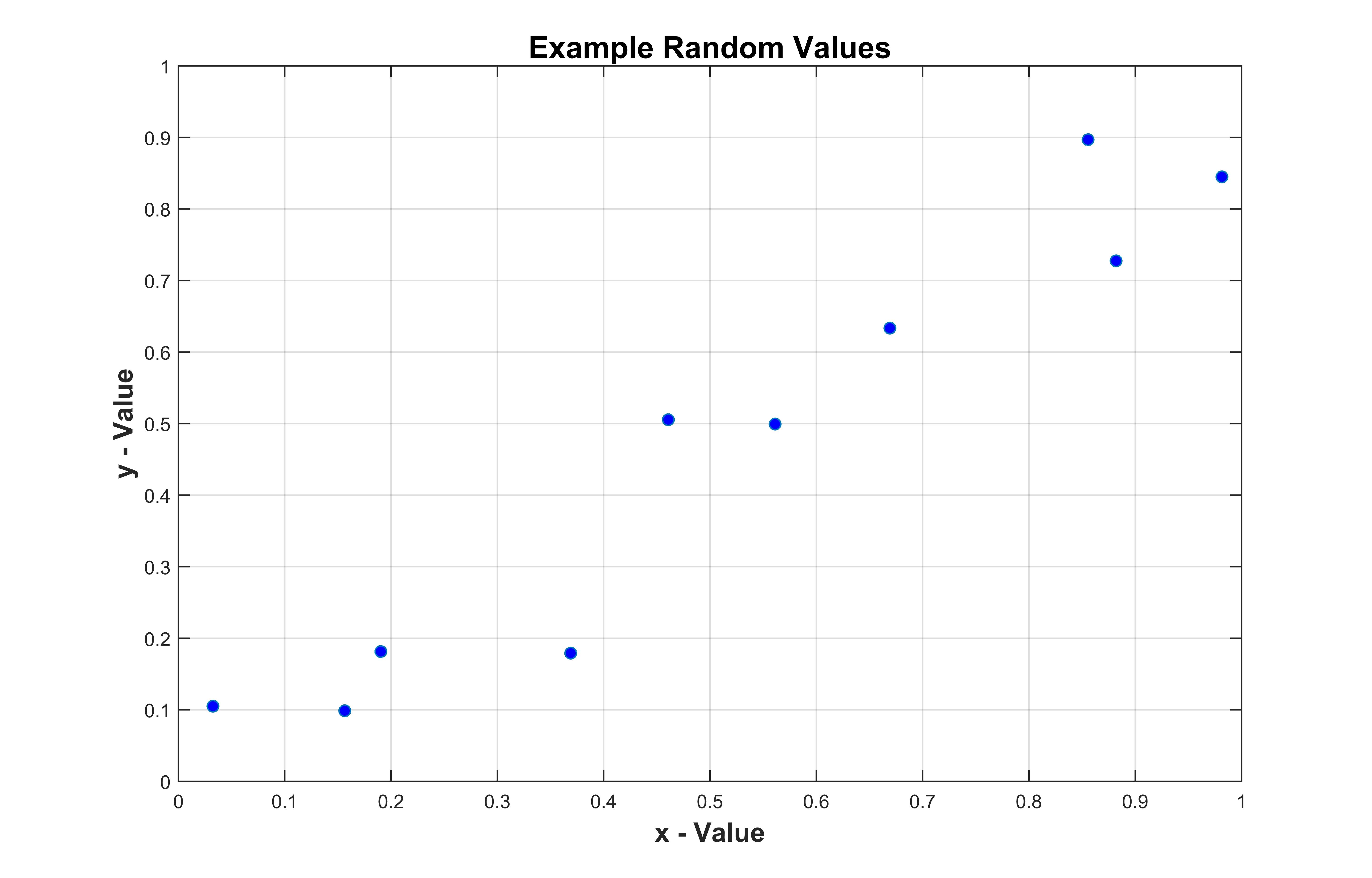
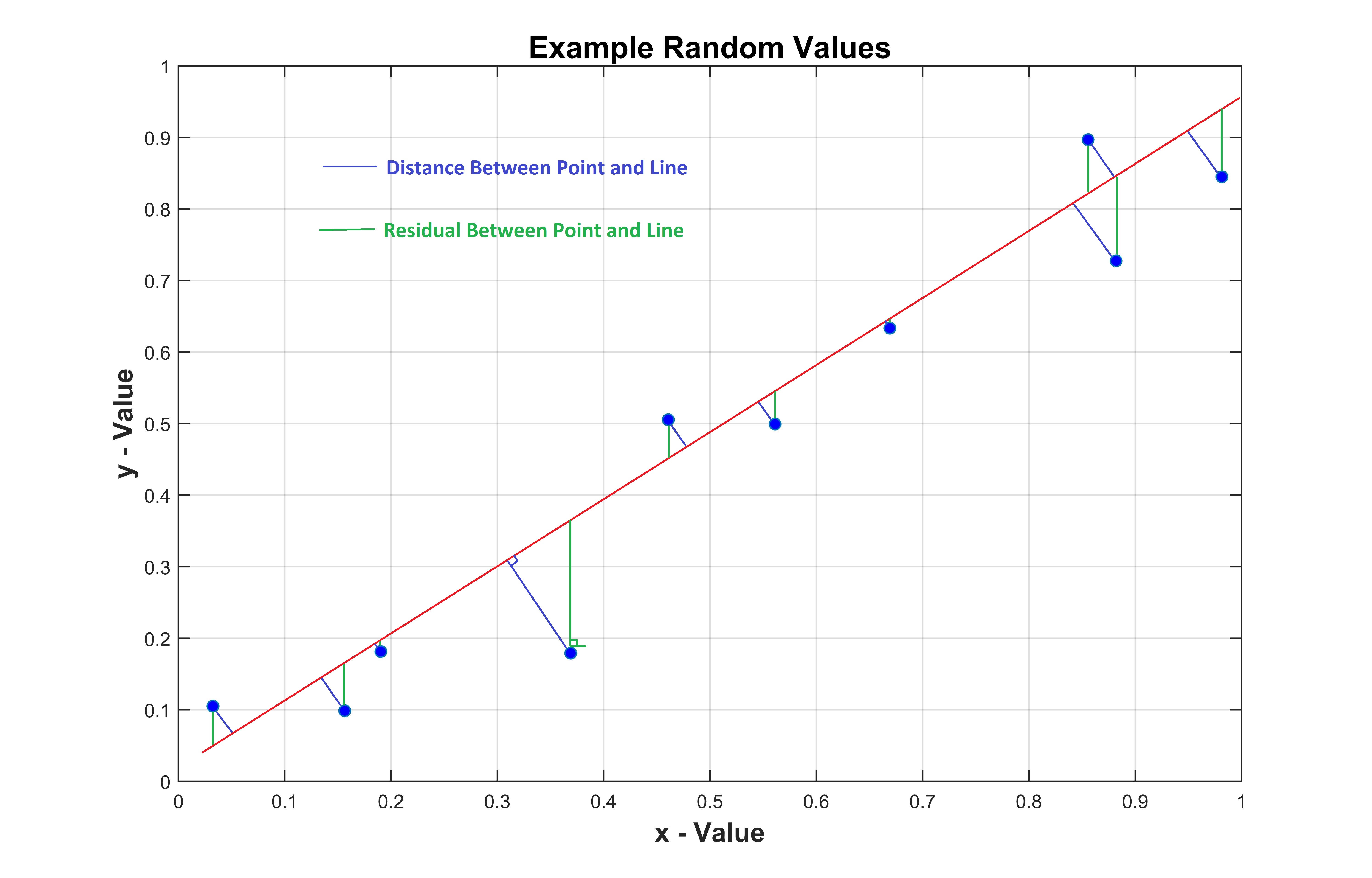
A reduction from two dimensions to 1 can be done by finding a "line of best fit". However, there are two predominant ways
to define this line. One can minimize the residuals (or the vertical distance between a line and the points), or one could minize the shortest
distance between the line and the points. When one minimizes the residuals (green), they are preferentially weighing error in a particular dimension.
This is illistrated in the figure below:
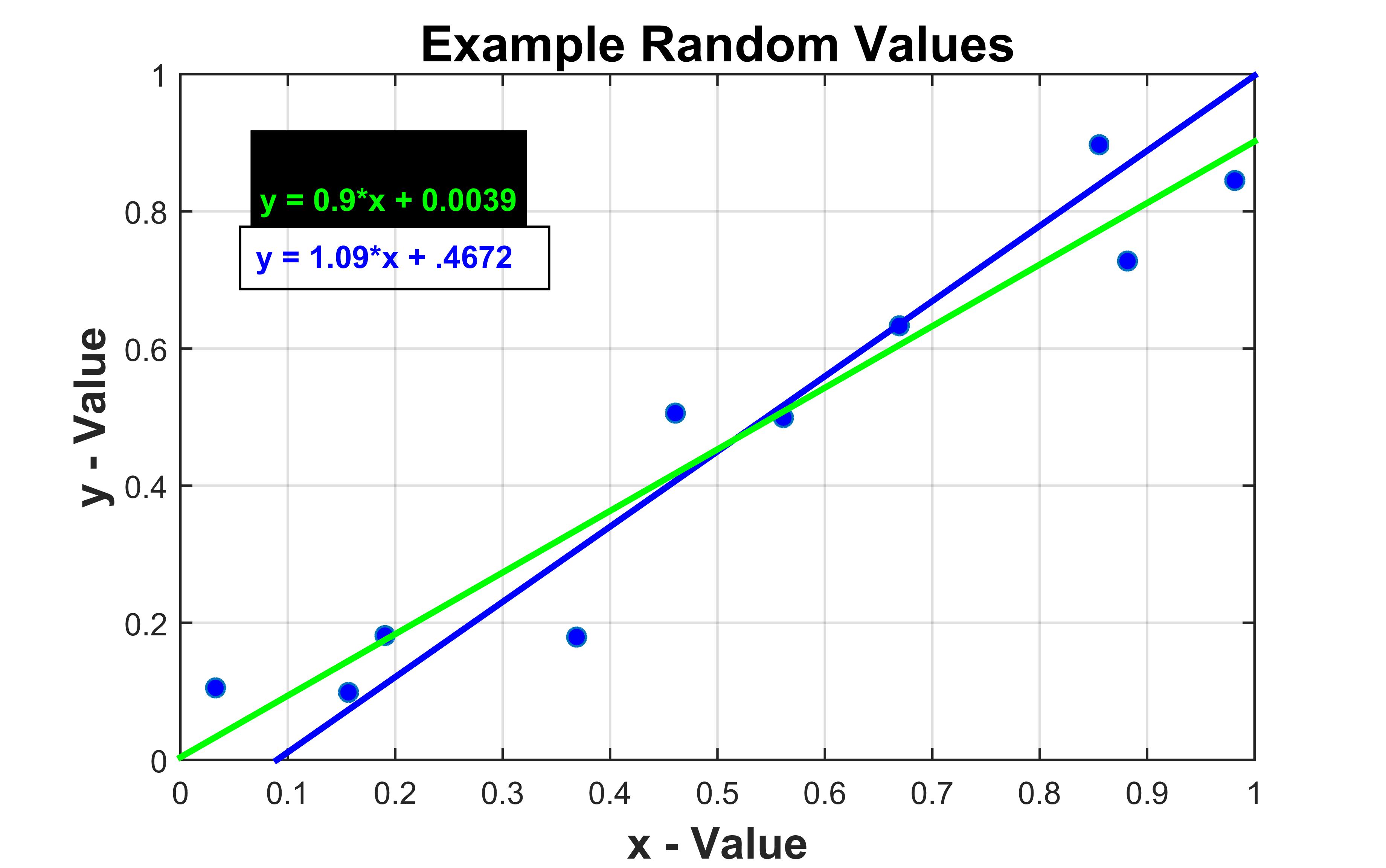
In general, these lines are different. An advantage of the residual method is if you know the x-values are right, and all the error lies in only one dimension. Another advantages is that the generalization of the residual method to any polynomial is simple. For our particular data-set, the lines are:
So, what about a harder problem?
We could consider if our data wasn't a straight line. In fact, we might even have a pathological case. Below is perhaps one of the most pathological cases, but there is a clear fit.

The generalization of this concept to higher dimensions is natural. Below is a 3-dimensional swiss role data set.
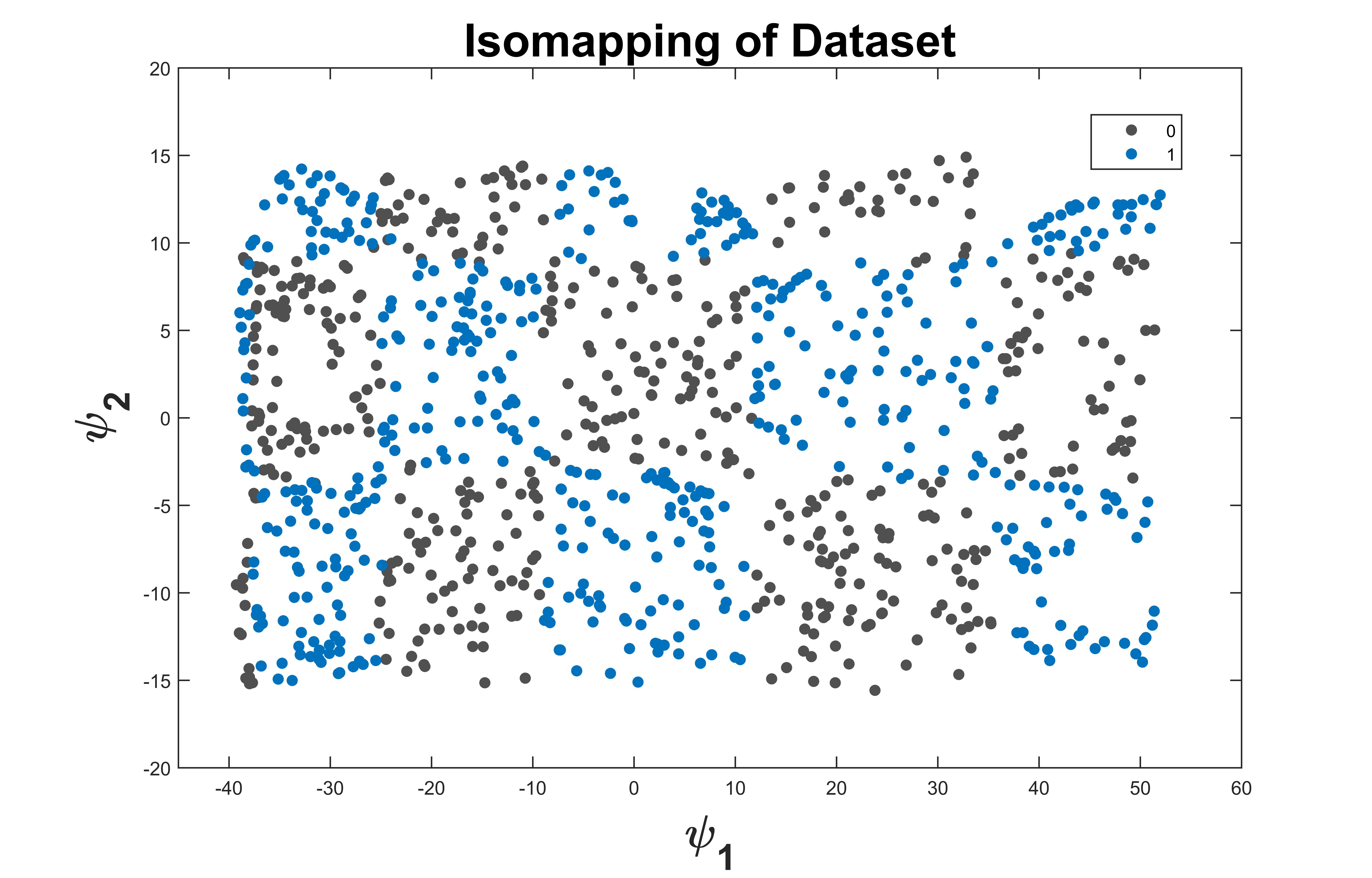
In the case of non-linear dimensionality reduction, the goal is to "unroll" the manifold. This is often viewed as:
Applications
It turns out it is practical to think of angle of rotation as a dimension (or parameter) which can characterize image data-sets. To justify this, I will
use our current MATLAB algorithim on a simple set of images.
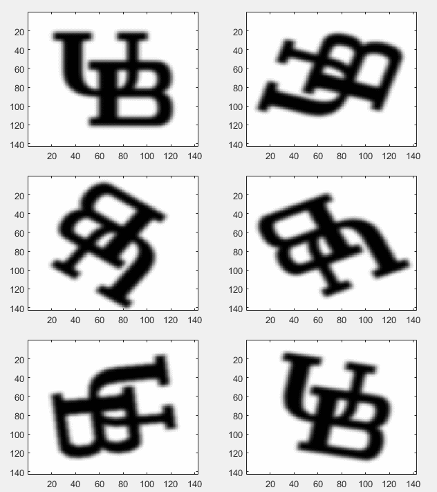
First, I will create a data set which is simply 300 rotated versions of the same image. This is seen in the GIF below
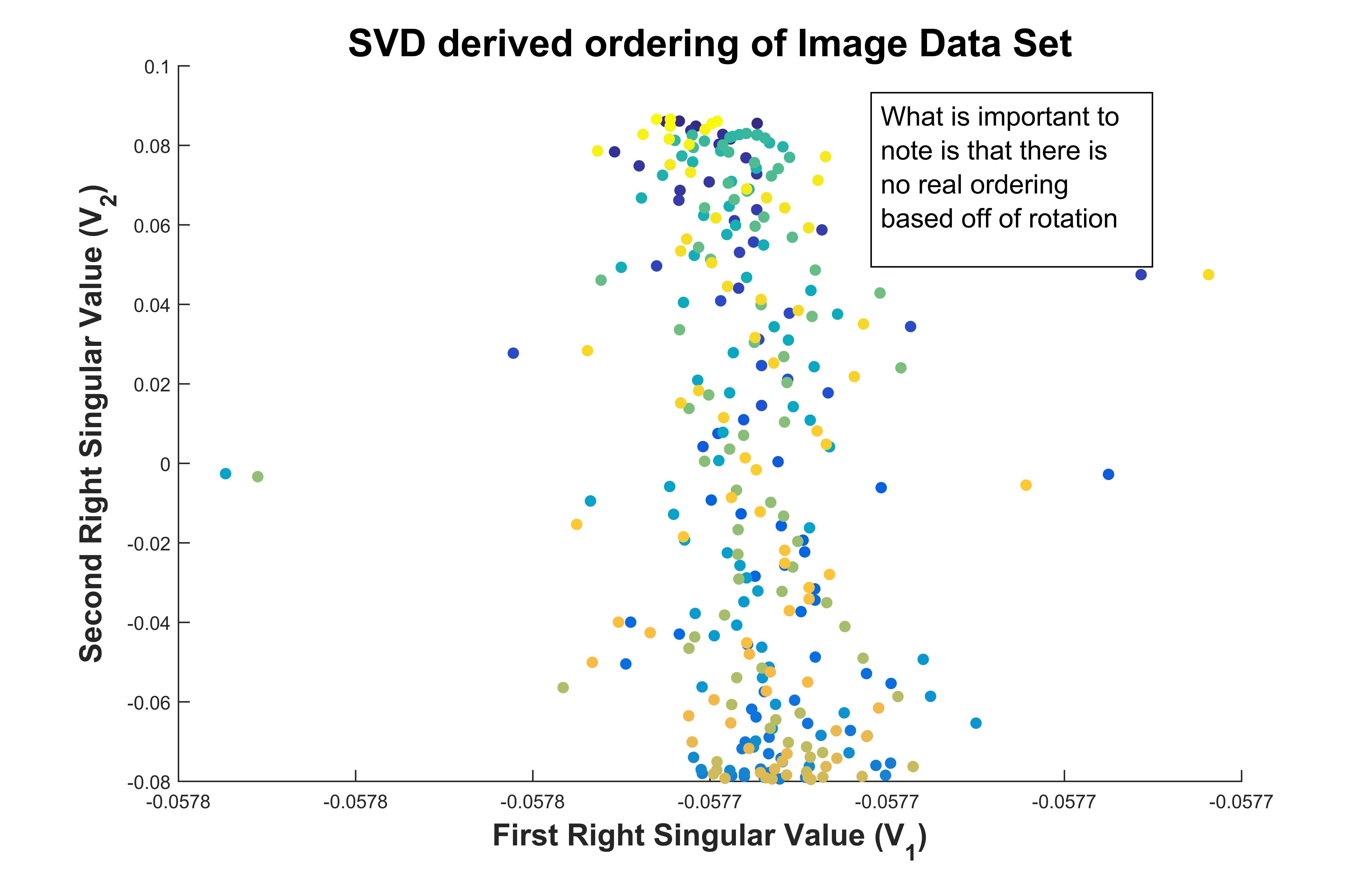
If I simply scatter-plot the first two eigen vectors of the data set against each other, and color the plot by rotation, it is easy to see that there is no correlation
However, it we use diffusion mapping on the data set and scatter plot the first two eigen vectors, the result is absolutely remarkable!
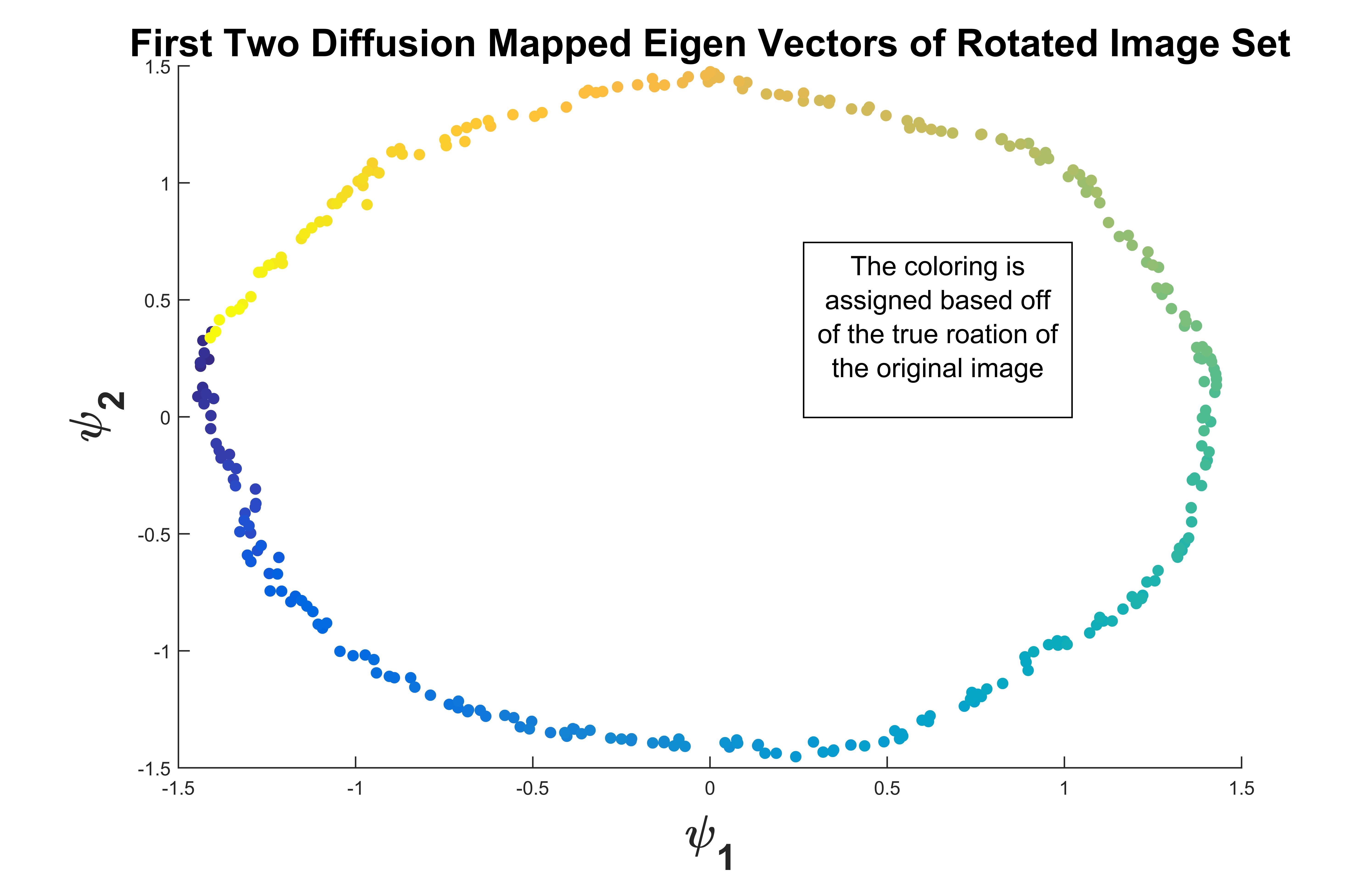
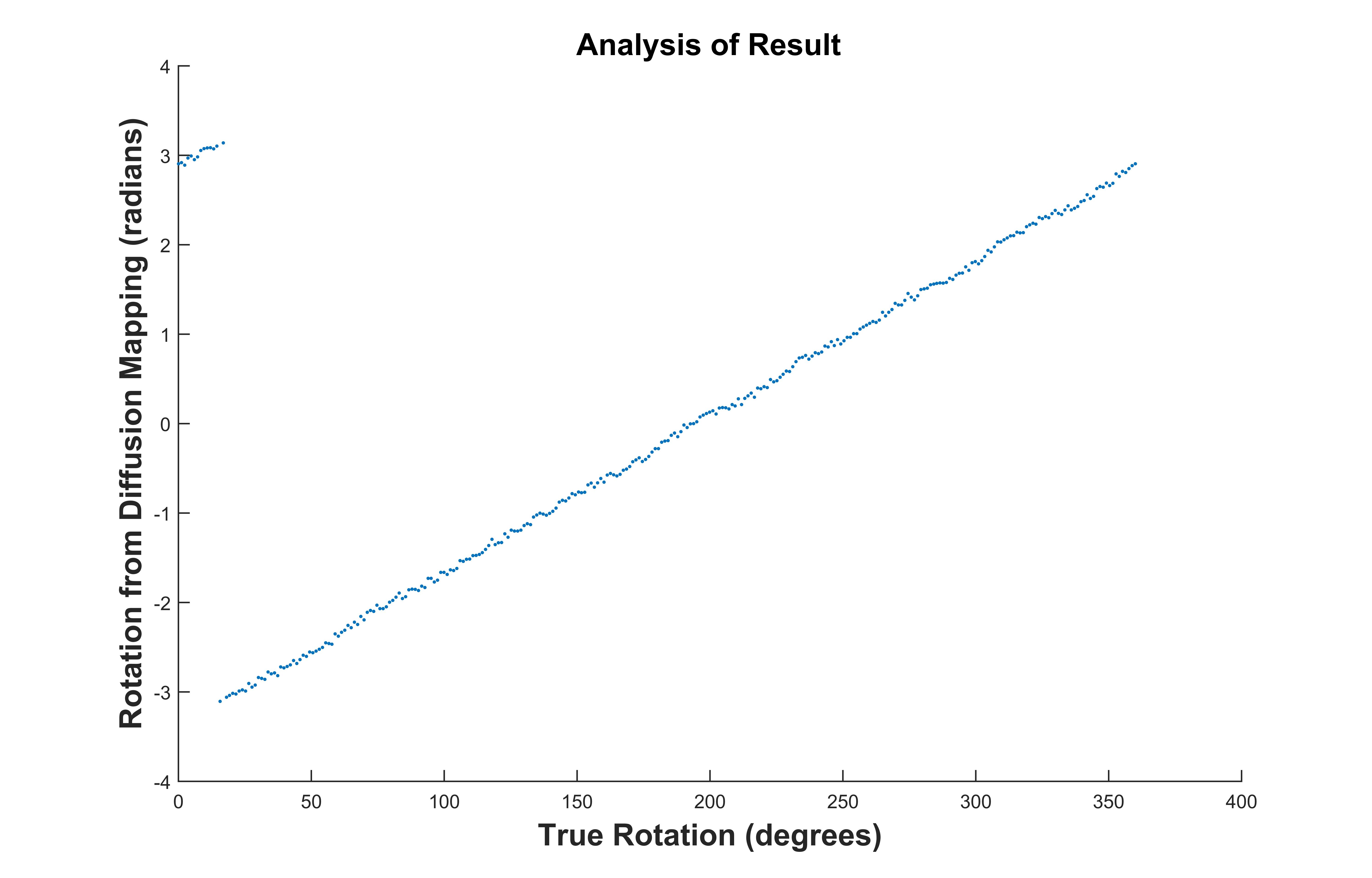
To check the accuracy, we can simply compare the true rotation to the angle found from the arctan of the first two eigen-vectors
